–by Robert L. Read and Sarah Abowitz
Let a supply chain network (SN) be a collection of people, places, inventory, designs and firms that are generally expressible in the OKF. For example, in response to a hurricane, a single city might create a supply chain network consisting of 5 microfactories, a large supply of raw materials, 25 skilled makers, and 10 trucks owned by the city. Mathematically, one can consider a supply chain network to consist of a set of material suppliers {MS1, ... , MSm}, a set of OKHs {OKH1, ... , OKHn}, a set of OKWs {OKW1, … , OKWo}, and a set of OKTs {OKT1, … , OKTp}.
Let a catalog (C) be a set of objects which can potentially be ordered. An important use case of this type is objects for which an OKH is available, although there may be other objects orderable. In general call objects which can be purchased without an OKH normal and those that require an OKH adaptive. This language is meant to express that the Open Knowledge Framework allows adaptation to and extension of a normal supply chain network when that normal supply chain network is disrupted or completely inoperable.
Let an order (O) be both a collection of items chosen from a catalog and a relation mapping said collection to to quantities to be delivered of each item. (Alternatively, an order is a bag or multiset from the catalog.)
Let a fulfillment plan (FP) be a document that maps an order into a supply network’s resources and connections between those resources that potentially can fulfill the order. If a supply network changes, it may invalidate a fulfillment plan that depends on said supply chain network. In general, a fulfillment plan references a supplier, an OKH, an OKW, and an OKT. Some fulfillment plans may be degenerate (for example, if a part is consumed in the same place that it is produced, it does not require an OKT.) (Note: Other elements of the Open Knowledge framework, such as OKM, may be referenced by the OKH and thus included by reference or transclusion, but are not directly part of the FP.)
A fulfillment plan is composed of a set of stages. In general these stages depend on the OKH that it mentions. Stages are either incomplete or complete. Each stage is something verifiable as complete by a human being, and may be annotated with documentation of a human assertion. Annotations of this kind should be sufficient to find the human agent that made the assertion of completeness. This level of documentation does not exist to assign blame or responsibility, but to take corrective action if the fulfillment plan is broken or if the assertion is later found to be inaccurate. The stages for a given object may be created from the OKH, or maybe generically created by the platform.
In general, a fulfillment plan moves from a state of unfulfillment to being fulfilled by means of stages being completed. Stages are related by a partial order relation, and when two stages are related in this way, we say one stage depends on another. Generally if stage y depends on stage x, it would be unusual for y to be complete and x to be incomplete, although there is nothing preventing a human from asserting that y is complete. This partial order creates a directed acyclic graph of stages called a stage graph. The ability to visually render this graph and its state of completeness is a useful feature of the platform.
A stage graph is a convenient object against which to perform a risk analysis. This may be considered a form of abstract interpretation as the term is used in programming language theory. For example, each stage could be annotated with a probability of (independent) failure at that node. The conditional probability of the fulfillment failing may then be computed directly from the independent probabilities of specific atomic failures. Because the probabilities of a stage failing may be highly time dependent, we can easily imagine different risk analyses based on different times.
A triple consisting of an order, fulfillment plan, and supply chain network (o, fp, sn) is a fundamental object supported by our platform. We may assume that an order, a supply network, and a fulfillment plan are implied by a dynamic supply chain and informally refer to this triple as a dynamic supply chain (D).
Let a platform sbe a semi-automated software system which, with the aid of humans, allows dynamic supply chains to be constructed and manipulated for the purpose of filling orders which actually deliver needed goods to people, even in the presence of supply chain disruptions. In actual practice, a supply chain network will be supporting a large number of dynamic supply chains at any one point in time.
A dynamic supply chain D is a mutable object which evolves over time, particularly as stages are completed. Dynamic supply chains may be indefinite, capturing the notion of continuous supply of some item across time, or definite in time, capturing the notion of an order being fulfilled and now closed. In order to understand the change of a dynamic supply chain over time, a dynamic supply chain has a history, which may be thought of as a function of the supply chain and time t which expresses the changes in a supply chain over time, which may be represented (H(D,t)). A dynamic supply chain which utilizes an element of an OKF is called adaptive. A dynamic supply chain which does not utilize the OKF is called normal.
Dynamic supply chains have the fundamental property of being recursively composable, as expressed in an example below where a dynamic supply chain for a chair is a composition of the dynamic supply chains for a back, a seat, and four legs. This composability fundamentally occurs at the stage we might call “delivery”. That is, if a part fundamentally relies on other parts, the delivery of those other parts may be considered an independent dynamic supply chain which is referenceable. Therefore, the dynamic supply chain for a chair may include by reference the dynamic supply chain for the seat. Although we may look at dynamic supply chains at different scales, for different purposes, we generally focus on the top-level dynamic supply chain which provides something useful to an end consumer.
A contract specifies a buyer and a dynamic supply chain. A contract may be potential, agreed upon/signed, contested or completed. We make no attempt to formalize the terms of the contract. Although contracts are very necessary for human cooperation, automating them is not necessarily to create a platform which provides useful supply chain interoperability.
In this sense, a dynamic supply chain is the fundamental data object that our platform and Open Knowledge Framework treats. Our proposed platform supports a number of functions listed below. It must be understood that at first, many of these functions are implemented with the assistance of real human beings solving real problems and making human judgements. Nonetheless, this is an organizing framework which should make supply chains more resilient. The framework may evolve through greater automation over time.
If we think of the platform as a computer program, it is similar to a database management system storing objects that are related to dynamic supply chains. However, it must provide some fundamental computational operations as well, and alongside those, some definitions of their set theory equivalents:
[A note from Rob: I’ve now read over this once and understand it. The big question in my mind now is if we should continue working at this level (a math-y level) or if we should work at a class-y level in Python. I’m going to try to understand Sage Math in Python a bit more before I make this decision. The work below is a good start. As a “theory” (in this sense of a collection of theorems, not in the sense of a question to be answered) it is weak because it presents no theorems. I also believe the symbol F is a big over used. Also I prefer not to use color because it is not supported by LaTeX and standard mathematical practice (I would prefer to use subscripts and different fonts to accomplish the intended distinctions.)]
[BIGGER NOTE from Rob: This work of Sarah’s was influential in the Python code that I wrote. However, the Python code now somewhat supersedes it by being more concrete. However, we now need to go BACK from the Python and into a Math-like notation as Sarah has used here. This will not be particularly difficult, and will cut down overall space here, but there is really no other way for us to proceed.]
For each S in SN:
If Type(S) == T:
If IsAnOKH(S):
K = the OKH for S
G = {}
For each input I in K:
G ⋃= {W(I,SN)}
F ⋃= P(T,K,G)
Else:
F ⋃= P(T,null,S)
return F
[Note: Rob is adding this section to record a thought that may be important; it is not yet unified with Sarah’s work above.]
In practice, the OKF augments rather than replaces existing supply networks. If we consider how an OKF-augmented supply network differs from a standard supply network, it seems that the fundamental action in an acute crisis is likely to be different:
Therefore, a fundamental operation is to produce a “negotiation frame” based on an OKH. The frame contains the contact information of all parties that most participate in the OKH: the maker, the suppliers of the inputs, and the buyer. This frame can then be used by either the maker or the buyer to understand prices and negotiate actual contracts allowing the delivery of the good to the buyer.
For example, suppose there is no supply of ready-made chairs, but an OKH for a chair exists. The fundamental inputs (at the first level of recursion only) to a chair are 1 seat, 1 back, and 4 legs. Let us assume that the supply network can provide seats, backs, and legs. The fundamental things a person who needs chairs wants to know are:
In turns out the price of a chair can be understood as an equation:
P = 4 * L + 1 * B + 1 * S + K = K + 4L + B + S,
where L is the price of a leg, B is the price of a back, S is the price of a seat, and K is a constant representing the price of the labor of assembly. Let’s name such equations the “characteristic pricing equation” of the fulfillment plan. Although all of these may be negotiable, the platform can give contact information for all of the people who can determine these prices with negotiation. So providing that info and the equation above is a fundamental operation. The Weave function does not technically have to produce the characteristic pricing equation because they can be computed from a fulfillment plan.
If more than one OKH is required (for example, nobody is supplying Legs but instructions for woodturning maple boards into legs are available), then naturally this becomes recursive. That is, an OKH may need an OKH to get a fundamental input. The characteristic pricing equation can be updated by simple algebraic substitution.
There is some opportunity for tiny amounts of linear algebra in this. If we think of the price of all basic inputs (fundamental inputs not created by OKHs) as a vertical vector P of length N and the number of distinct goods purchased in an order by M, then we can compose the characteristic equations into an M-row, N-column matrix Q. The price of the order is a vertical vector of length M defined by the matrix multiplication of Q x P. (The total price is the L1-norm or simple sum of P.)
Although elegant, this has limited utility, because in general Weave should produce multiple plans for obtaining a given good. Until a plan is chosen, the matrix approach cannot be used by simple multiplication (it can still form a useful “table” however.) However, if one sets aside the multiple plan problem, then one can even form a “Price Jacobian” as a matrix which gives the change in price of the final good as a function of the change in price of the input fundamental commodities. This could be used to compute the points in which two plans for the same good have equal total prices based on commodity prices.
In general, prices will be set by the actions of (human) agents who are both buying and selling. This is especially true in a disrupted supply network, when the fundamental assumption of perfect market knowledge is unlikely to hold. Therefore any discussion of pricing will be somewhat academic. Nevertheless the characteristic pricing equations remain useful as an incontrovertible minimum price.
One of the advantages of the characteristic pricing equation is that it delays making a decision if prices are treated as continuous or discrete. For example, many firms wish to establish a supply chain that constantly, continuously, and smoothly delivers goods. In such a situation demand and supply need not be measured in absolute units but as rates---units per unit time. For example, ventilators per day. A given firm may only be able to make 2.7 ventilators per day. The fact that a fraction of a ventilator is nonsense is irrelevant so long as the orders are large and long-duration.
Discrete pricing, on the other hand, imagines the fulfillment plan as executing a single operation and then stopping.
Note: Our current OKF probably does not assign unique enough identifiers of the “type” of the good. This is the domain of so-called ontologies. This problem is neither completely solvable, nor particularly problematic---we can survive doing this by hand in many cases.
Dynamic supply chains have the properties of composability and recursive definition. The OKF supports this, though not without some human interaction. For example, to make a chair, you may need legs, a seat, and a back. Let us suppose that a given microfactory allows the construction of a dynamic supply chain (L). For the time being, assume this is elementary–that we need not consider what goes into making legs, but can trust that our supply chain network provides a factory that can make legs. An order O(L) can create a dynamic supply chain that delivers legs.
Likewise, if we can make a seat (S) and a back (B), we can compose instances of these three objects to make a chair (C). An oversimplification in terms of objects which may be chosen from the catalog of the OKF is: C = 4L & S & B.
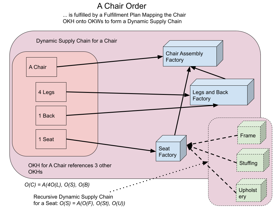
Figure 4. A diagram of the recursive dynamic supply chain for a chair, which also contains a recursive dynamic supply chain for a seat.
In actuality, a dynamic supply chain which fulfills legs can be composed with dynamic supply chains for a seat and back to create a dynamic supply chain for a chair. An order for a chair can be fulfilled against this dynamic supply chain.
Of course, a chair is not just a box containing four legs, a seat and a back. These objects must be fitted together and assembled, and this operation can fail. Technically, we would say:
O(C) = A(4O(L), O(S), O(B))
where A is a function of assembly coming specifically from an OKH template.
This structure is a tree of depth 1. In actual practice, a dynamic supply chain would likely be deeper. However, we can generally compose dynamic supply chains in tree-like fashion of expanding depth. The function A is not quite so simple as a pure union of subsets, but we can usefully pretend this is so to organize a dynamic supply chain.
When we discuss the completeness of dynamic supply chains below, we mention the concept of a property such as being free of the allergen latex. We can define a boolean function F operating on dynamic supply chains that represents allergen-freedom, which can literally be defined recursively:
F(P) = human assertion, when P is an elemental part
F(A(P1,P2,...PN)) = F(A) && F(P1) && F(P2) … F(PN)
Like completeness, allergy freedom is a computable function against fulfillment plans.
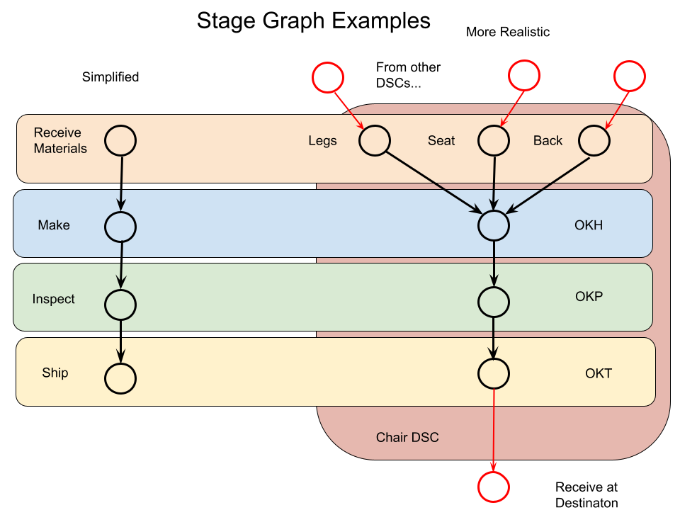
Consider what the stage graph of the dynamic supply chain for the chair might look like, as shown in the figure below. A very simplified graph might have four stages: Receive Materials, Make, Inspect, and Ship. However, a platform that is expected to be useful, particularly in the presence of widespread disruptions and chaos, should provide richer tracking, as shown on the right of the figure. This diagram also suggests the composition of the dynamic supply chains.
One aspect of modularity boils down to this: When is it acceptable to replace a part P with a similar part P1? For example, for a given order for a chair O(C) using a back B, how do we know a similar design for a back B1 is an acceptable replacement? A supply network which allows this substitution is generally more resilient than one which does not. Even if it requires human judgment, a recursive structure is more comprehensible when explaining such modularity to others.
For example, let us suppose that a buyer has used the platform to generate a dynamic supply chain for a chair and the order has been placed. The platform formally tracks this status of O(C) = A(4O(L) ⋃ O(S) ⋃ O(B)) as “placed”. The order is a witness to the agreement of the parties to build and deliver a chair.
Now, suppose there is a supply network rupture, and the manufacturer of seats cannot fulfill their part of the order. However, there is a seat S1 in the catalog. We do not imagine that S1 can be substituted for S without human approval, but the order allows the means for one to ask the buyer if S1 is an acceptable replacement to S, and for one to record said answer. The resilience of the supply network improves as more components, such as seats, are added to the OKF.
Let modularity be the replacement of one object for another. Composability is a more powerful concept: it is the ability to rearrange the relationships between objects. The platform supports the composability of dynamic supply chains, but not objects. For example, we might have a supply network comprising three microfactories, one making legs, one making seats, and one making backs. However, if one of these is removed from the supply network by a mishap such as a flood, we must now compose a dynamic supply chain using only two factories. Some factories will have to make more than one kind of component if we are to fulfill an order for chairs. However, this is possible and anticipated by factories that can process a wide variety of OKHs.
A interoperable dynamic supply chain is created when someone establishes a platform that uses the OKF. Such a dynamic supply chain can be thought of as the elements that fulfill an order. For example, one can easily imagine an OKH being created very quickly in response to an emergency which is quite specifically tailored to ensure the device is manufactured in a way that meets FDA requirements, whether those are long-standing or were created acutely through an Emergency Use Authorization. An order is complete when there is verifiable evidence that a dynamic supply chain can fulfill the order. Although this evidence may be automated in some cases, it will generally consist of recorded human assertions.
If we consider a general order purchasable from the catalog presented by the platform, the object will automatically have quality assurance built into the OKH, instructing how to build and verify it. However, suppose that the buyer purchases new requirements or criteria on the order, such as that it be latex-free or nickel-free, which is not already a part of the OKH. A human being can create evidence that the object is allergen-free by checking the OKMs of all the ingredients that comprise the object. This evidence, in combination with the rest of the OKHs’ tests, may make this order complete in the context of a dynamic supply chain which can provide all the components necessary to fulfill the order.
Checking for completeness of orders and composing orders which are complete is the primary executable function of the platform. We may expect this evidence to be generally correct, but occasionally humans make errors. In that case, the order will not be properly fulfilled; however, the failure is any understood in the context of the traceability of the error. The OKF and traceability provide all the information necessary to track the problem down and fix it. For example, the evidence that no sub-component contains nickel could have been made erroneously even though a sub-component clearly states that it contains nickel, or alternatively, a component may contain nickel while erroneously stating that it is nickel-free. There may be other failure modes, but the platform, the dynamic supply chain, and the OKF, provide means of addressing the problem. The order, although not fulfilled, still represents a useful correctable plan for its fulfillment.
Physical objects produced by the OKF are composable. Often to supply an object dynamically, a supply chain must supply several components. Each of these components may be thought of as requiring an order fulfillment against a dynamic supply chain.
A quality criterion can be recursively verifiable by being verified by each dynamic supply chain which makes a part of a product. Freedom from allergens is such an example; if all components are allergen free, the product is allergen free. In general, however, each quality criterion is not so easy to satisfy with simple evidence. Nonetheless, the OKF provides at least a framework for providing evidence of completeness. For example, suppose that two materials are heat-bonded into a mask. The platform likely has clear quality controls on each material separately, but is not expected to be able to assert that they can be heated in contact without producing a toxic byproduct. However, a human being can provide this evidence at the level of the final product (which may be only a sub-product from the buyer’s point of view.) This framework thus provides an evidentiary record of the completeness and satisfaction of all criteria, even though this is not fully automatable and is subject to human judgment and error.
An order can be thought of as a sentence or expression in an informal language, which can be checked for completeness by checking that the platform and dynamic supply chain and assembly processes can provide a product which meets all criteria. A provably complete order is a good candidate for fulfillment. Although quality, production capability, and ability to finance the operation are all required to complete the order, it may be useful to separate these concerns. For example, an order may be complete, yet also rely on a manufacturer of a sub-component in a microfactory with no established reputation. The buyer may then hesitate because they are not convinced that every needed component can be reliably supplied by the dynamic supply chain. This unreliability is partially addressed by the fungibility of resources provided by the OKF. If an agile, dynamic supply chain is established, one manufacturer may indeed be statistically unreliable, not because of quality but simple failure to execute obligations. However, the OKF provides inherent resilience in that the unreliable party is not the only party which is capable of making the subpart, by definition. Although a failure of one supplier may delay a specific order, the order can be successfully completed by other suppliers from the OKF. Thus the OKF allows resilient, composable dynamic supply chains to be established which allow orders to be checked for completeness, and provide the ability to trace and recover from failures of the platform.
Note: The following assumes price affects neither supply nor demand. This is appropriate for life-critical equipment in the presence of supply shortages. Equivalently, the demand and supply are both highly inelastic.
Let the symbol B represent fragility. The units of B could be human mortality or morbidity, but it is probably most convenient to use dollars as the unit. Note: The value B may be thought of as “lost value due to fragility”. It can exceed the total value spent on a particular product because it can measure surplus value. For example, if toilet paper is $1 before a crisis and then is in short supply and the price would naturally rise to $10/roll, the surplus value of toilet paper, even when the price is $1, is clearly $10.
Let Sp(X) be the maximum number of units that a group of suppliers X can provide of product p.
Let Wp(D,S) be a weighting function of the demand D for p and the supply of S of p. W can be any function desired producing the same units as fragility, with two conditions: W is decreasing in S, and increasing in (D-S).
Acceptable examples of W are:
Wvent = $50K * { Dvent - Svent, if Dvent < 100K;
100,000 - Svent, if Dvent >= 100K}
Wmask = $5 * { 0, if Smask < Dmask;
(Dmask - Smask) / Dmask , else}
Let Pp(d) be a probability density function representing the probability of a specific demand d for product p.
The B is the expected fragility of a set of suppliers Y is the integral over all demand products (p) over all probabilities x:
Let B represent the expected fragility of a set of suppliers Y. We define this by integrating over the probability distribution P of all possible demands (x) for all products (p).
B(Y,Pp,Wp) = ∫p ∫xWp(Dp,Sp(Y)) Pp(x) dp dx
We can then make some useful and logical conjectures on the nature of fragility in SCIS.
Conjecture 1: Increasing the set of suppliers does not increase fragility. Let A be a set of additional suppliers to the set Y.
B(Y ⋃ A, P, W) <= B(Y, P, W)
Under suitable assumptions of W and P we can prove much stronger theorems.
Actual values of B can be computed by Monte Carlo simulation (based on probability distribution). The utility of these values will be based on the realism of the variables.
Note: (Kevin wanted me to add this language)
The purpose of your platform is to allow delivery of needed goods when all of the trust mechanisms that are normally in place have been dissolved because of an extraordinary supply chain disruption. Normally, a buyer does not need to worry about a fulfillment plan---that is handled by professional procurement officers in normal circumstances. However, during an emergency, the buyer may want and need to see an entire fulfillment plan in order to have confidence that their demand can be met.
A graph is only as resilient as the count of its separable paths. The convergence of independent paths through a supply graph is often called a bottleneck. A supply graph’s resilience metric is reducible to an evaluation of its bottleneck, in units of important metrics like agility (rise time to meet new demand signal).
Individual paths through a supply graph may converge, or diverge from, these bottleneck points. Formally, a path is separable from another path, if they share no nodes (and consequently no edges).
Example 1: There might be 10 routes home, but all take the bridge. Therefore there is one route home. The routes share an edge (the bridge) so they are not separable and all routes are subject to the same stress failures.
Example 2: TMSC produces 54% of the global supply of semiconductors, so 54% of products containing electronics could be assumed (*unless components are recycled from previous stock) to be connected upstream to that production node, and therefore influenced by shocks to it. Furthermore, ASML produces the ultra-specialized photo-lithography equipment in use by all semiconductor fabs, so the supply of
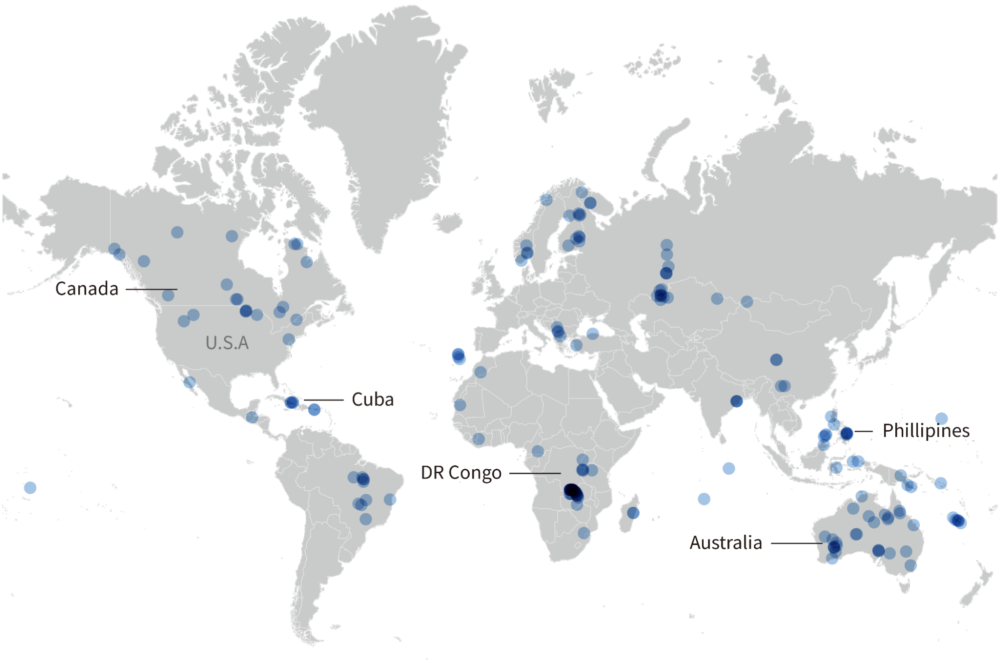
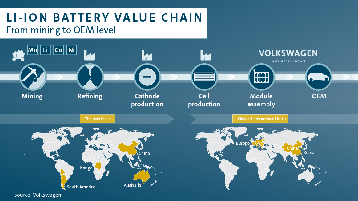
Example 3: Lithium production process example from Volkswagen.
Figure: Global map of lithium mines. If a product contains lithium, it must have originated, at some point in history, from one of these locations.
Figure: Lithium to end use in cars. This represents the highest-level (“chunked” -- see Hofstadter) abstract transformation pathway. In order for this to be actualized, it must be instantiated by real production facilities. If any node in the pathway is shared by all upstream facilities, that node is a point of failure.